Distributions

Simple distributions

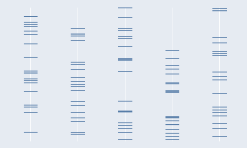
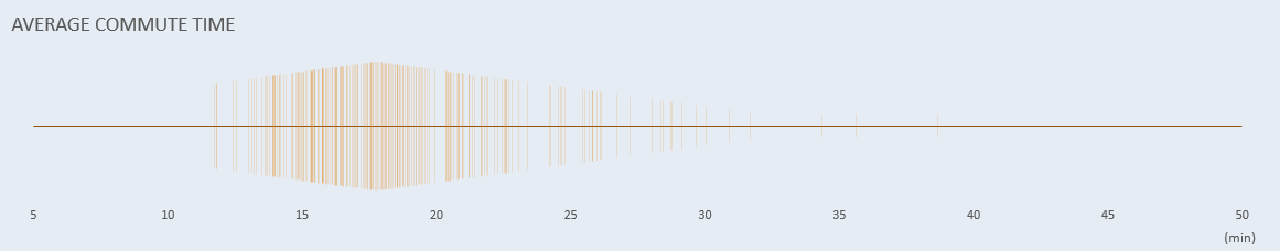
For each variable, entities (or observations) can assume a wide range of values. We can encode those values and visualize them along an axis and search for (lack of) symmetry in their distribution, compactness, or outliers. Since data points are usually not labeled, the display can be remarkably compact:

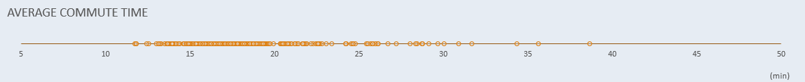
With too many data points, overlaps are unavoidable. You can try different techniques to minimize them, like jittering, whereby you add a small amount of random noise to the opposite axis:

I used a vertical line instead of a circle, then added some transparency, and the central value is the median.

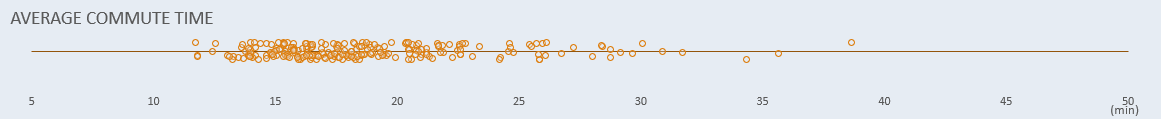
Here is the same char with many more data points:

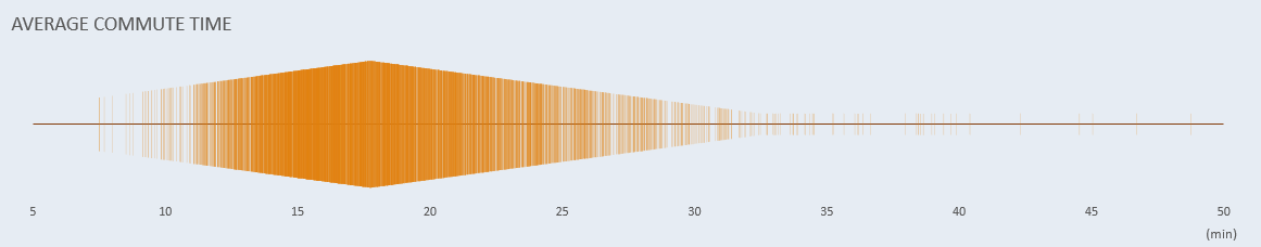
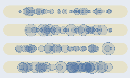
You can split the distribution along the y axis or encode meaningful data into other visual variables, like color or size.

Summarizing the distribution by y-axis section

Often you don’t need all this detail. You need a few pointers (quantitative, visual) summarizing the distribution’s shape while losing as few details as possible. The most radical pointer is a measure of central tendency, like the mean, or average. In the chart above, there are 4260 data points, with an average of 18.6. We now have a reference value, but it tells us nothing about the distribution shape: is it compact? Is it symmetric? If we add that the standard deviation is 4.6, we can say that a value between 14 and 23 min is very plausible. The more pointers we use, the more detailed the picture is.

A somewhat different approach is to take the entire axis and split it into sections (called “bins”), counting the number of data points in each one. That’s what we do when making a histogram.

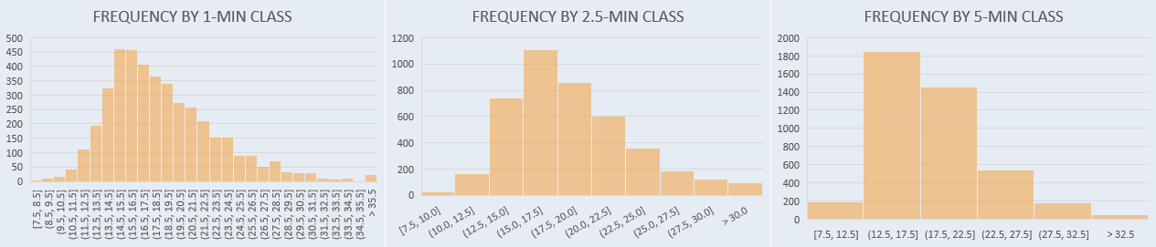
As you can see, higher resolution (shorter sections) creates a more detailed histogram, but all that detail can be unnecessary for the task at hand. If you define larger bins, you get the opposite problem: some useful information will be lost. Defining bins is a balancing act that needs to consider the shape of the distribution, the nature of the data, and the context.

Summarizing the distribution by counting data points first

Instead of applying pre-defined cut-offs and counting the number of data points in each section, we can go the other way around: after sorting the data, create groups with an equal number of data points and see where those cut-offs fall. If we split it in two, the cut-off point is the median, and if we split it in four, we get quartiles. Or you can create customized cut-offs that make sense for your data or the task at hand.

As you can see below, 50% of all cases fall between a little above 15 and 21. So you can say this is the standard commute time. You could then do something like multiplying the normal range by 1.5 and use this new range to add two new sections that help you evaluate the distribution’s symmetry and compactness. All data points that fall outside this extended central range are outliers.

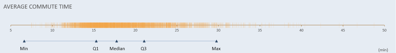
In many cases (not all), this is enough to describe the distribution with an acceptable loss of information. So we can use a box-and-whiskers plot:

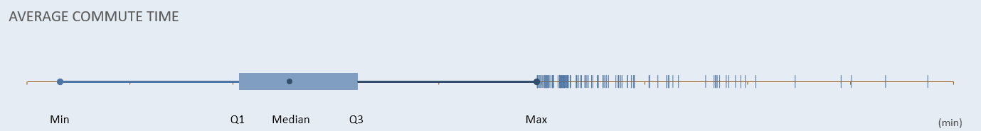
The box-and-whiskers plot removes the data points and replaces them with the cut-offs. Outliers remain visible because they are assumed to be relevant.

Takeaways

Distributions are often too complex to be summarized faithfully by common statistical indicators. Visualizing them gives us a better sense of their shape and helps validate the chosen statistical indicators: the median is often a better measure of the mean when dealing with skewed distributions, but that’s easier to grasp using a chart. (The Anscomb Quartet explores how charts and statistical measures complement each other.)

The most popular charts for summarizing a distribution are histograms and box-and-whiskers plots. Histograms are more intuitive, but bins must be carefully defined. You can avoid that somewhat subjective step using box-and-whiskers, which also have a standard formula to identify outliers. However, some distribution shapes can give misleading results, like a bipolar distribution around the median.

By the way, if you don’t have too many data points, strip plots can also be used instead of bar charts. Check Categories and Ranking.

Tutorials

---